Model Predictive Control Part I: Sufficient conditions for safe policy synthesis
Model Predictive Control (MPC) is an established control methodology which systematically uses forecasts to compute control actions. This control methodology is ubiquitous in industry, with applications ranging from autonomous driving to large scale interconnected power systems. MPC owes its popularity to the simplicity of the control design, which allows the controller to naturally account for both state and input constraints. In this post, we are going to discuss sufficient conditions for designing safe MPC policies, which guarantee constraint satifcation and closed-loop stability.
The Control Problem
First let’s introduce the control problem that we aim to solve. Informally, the goal of control synthesis is to design a policy which guarantees safety and optimal performance for the closed-loop system. These objectives can be often described by a dynamic optimization problem. For instance, consider a dynamical system governed by the update equation \(x_{t + 1} = f(x_t, u_t)\), where the control input \(u_t \in \mathbb{R}^{d}\) and the system state \(x_t \in \mathbb{R}^{n}\). For a control task starting at \(x(0)\), the control policy should apply to the system the optimal sequence of inputs \(U_T^* = \{u_0^*, u_1^*,...\}\) solving the following infinite time optimal control problem:
\[\begin{align} J^*(x(0)) = \min_{u_{0},u_{1},\ldots} \qquad & \sum_{t=0}^{\infty} h(x_{t},u_{t}) \label{eq:FTOCP_RunningCost}\\ \textrm{subject to:} \quad & x_{t+1}=f(x_{t},u_{t}), \forall t\in \{0,1,\ldots\}\\ &x_{t} \in \mathcal{X},u_{t}\in \mathcal{U}, \forall t\in \{0,1,\ldots\} \label{eq:FTOCP_TaskConstr}\\ & x_0=x(0). \end{align}\]In the above dynamic optimization problem, safety is naturally encoded through the sets \(\mathcal{X}\) and \(\mathcal{U}\), which represent state and input constraints. Finally, the performance of the closed-loop system is quantified by the running cost \(h(\cdot, \cdot)\) which we would like to minimize.
Predictive Control
For a particular task starting from \(x(0)\), one may be tempted to solve Problem \(J^*(\cdot)\) and apply the optimal sequence of control actions to the system. There are two difficulties associated with this idea. First, the infinite (or long) duration of the task can easily render the solution to Problem \(J^*(\cdot)\) hard to compute. Second, the model \(f(\cdot)\) used to predict the evolution of the real system can be inaccurate, and even small prediction errors which cumulate at each time step can compromise the success and/or optimality of the closed-loop behavior. To alleviate both issues, it is common practice to \((i)\) solve a control problem over a horizon \(N\) shorter than the task duration and \((ii)\) continuously measure the state of the system, say once every time step, and then recompute new control sequences with updated information from the environment. Commonly, the procedure we have described above is referred to as \(Model\) \(Predictive\) \(Control\) \((MPC)\). At the generic time \(t\), an MPC policy solves the following problem:
\[\begin{align} J^{MPC}(x(t)) = \min_{u_{0},\ldots,u_{N-1}} \qquad & \sum_{k=t}^{t+N-1} h(x_{k},u_{k}) + V(x_{t+N}) \\ \textrm{subject to:} ~~\quad & x_{k+1}=f(x_{k},u_{k}), \forall k \in \{ t,\ldots, t+N-1 \} \\ &x_{k} \in \mathcal{X}, u_{k}\in\mathcal{U}, \forall k \in \{ t,\ldots, t+N-1 \} \\ &x_N \in \mathcal{X}_N, \\ & x_0=x(t). \end{align}\]where \(x(t)\) is the measured state at time \(t\).
Let \(U_N^* =\{u^*_{0}(x(t)),\ldots,u^*_{N-1}(x(t))\}\) be the optimal solution to the above problem at time \(t\). Then, the first element of \(U_N^*\) is applied to the system and the resulting MPC policy is:
\[\begin{align} \pi^{MPC}\big(x(t)\big)=u^*_{0}(x(t)). \end{align}\]In the above equation we use \(u^*_{i}(x(t))\) to emphasize that the optimal solution depends on the current state \(x(t)\). Later on, whenever obvious, the simpler notation \(u_i^*\) will be used. At the next time step \(t+1\), the optimization problem \(J^{MPC}(\cdot)\) is solved again based on the new state \(x(t+1)\), yielding a \(moving\) or \(receding\) \(horizon\) control strategy. We point out that it is important to distinguish between the real state \(x(t)\) and input \(u(t)\) of the system at time \(t\), and the predicted states \(x_t\) and inputs \(u_t\) in the optimization problem.
Compare the MPC problem \(J^{MPC}(\cdot)\) with the original control problem \(J^*(\cdot)\) that we want to solve. The MPC problem \(J^{MPC}(\cdot)\) is solved over a shorter horizon \(N\), and it uses a terminal cost \(V(\cdot)\) and terminal constraint set \(\mathcal{X}_N\) to “approximate” cost and constraints beyond the perdition horizon, i.e., from time \(t+N\) to completion of the control task. The choice of the terminal cost \(V(\cdot)\) and terminal constraint \(\mathcal{X}_N\), which are often referred to as \(terminal\) \(components\), are critical in MPC design.
The Importance of the Terminal Components
It is clear that the prediction model plays a crucial role in determining the success of MPC policies. If the prediction model is inaccurate, then the closed-loop system will deviate from the MPC planned trajectory. This deviation may result in poor closed-loop performance and safety constraint violation. It is less obvious that, when a perfect system model is used to design an MPC policy, the wrong choice of terminal constraint set and terminal cost function may cause undesirable closed-loop behavior.
Recall that the MPC problem \(J^{MPC}(\cdot)\) plans the system’s trajectory over a horizon of length \(N\), which is usually much smaller than the task duration. With short horizon \(N\) the controller only takes shortsighted control actions, which may be unsafe or may result in poor closed-loop performance. For instance, in autonomous racing a predictive controller that plans the vehicle’s trajectory over a short horizon without taking into account an upcoming curve, may accelerate to the point that safe turning would be infeasible. In this example, shortsighted control actions would force the closed-loop system to violate safety constraints. Furthermore, shortsighted control actions may lead to poor closed-loop performance. Consider an autonomous agent trying to escape from a maze along the shortest path, a predictive controller may take a sub-optimal decision, if the short prediction horizon does not allow the controller to plan a trajectory which reaches the exit.
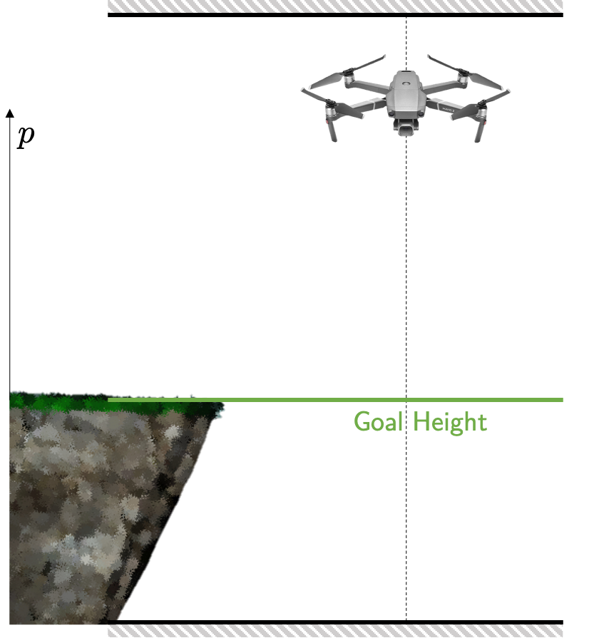
Next, we illustrate on a numerical example that shortsighted control actions result in unsafe or poor closed-loop behaviors. We consider the drone hovering problem, where our goal is to control a drone that can move only along the vertical axis. In particular, the objective of the controller is to steer the drone at the same height of a nearby cliff shown in the following figure.
In this example, the system dynamics can be approximated by the following double integrator system
\[\begin{align} x_{t+1} = \bigg[ \begin{matrix} 1 & 1 \\ 0 & 1 \end{matrix} \bigg] x_t + \bigg[\begin{matrix} 0 \\ 1 \end{matrix} \bigg] u_t \end{align}\]where the state \(x_t\) collects the position of the drone along the vertical axis \(p_t\) and the velocity \(v_t\), i.e., \(x_t = [p_t, v_t]^\top\). The input \(u_t\) represents the acceleration command that may be used to change the drone’s velocity at the next time step. The above system is subject to the following state and input constraints
In order to regulate the system to the origin, we implemented the MPC policy without a terminal cost and constraint, with \(Q = I\), \(R = 100\) and for different horizon lengths \(N \in \{3,4,5\}\).
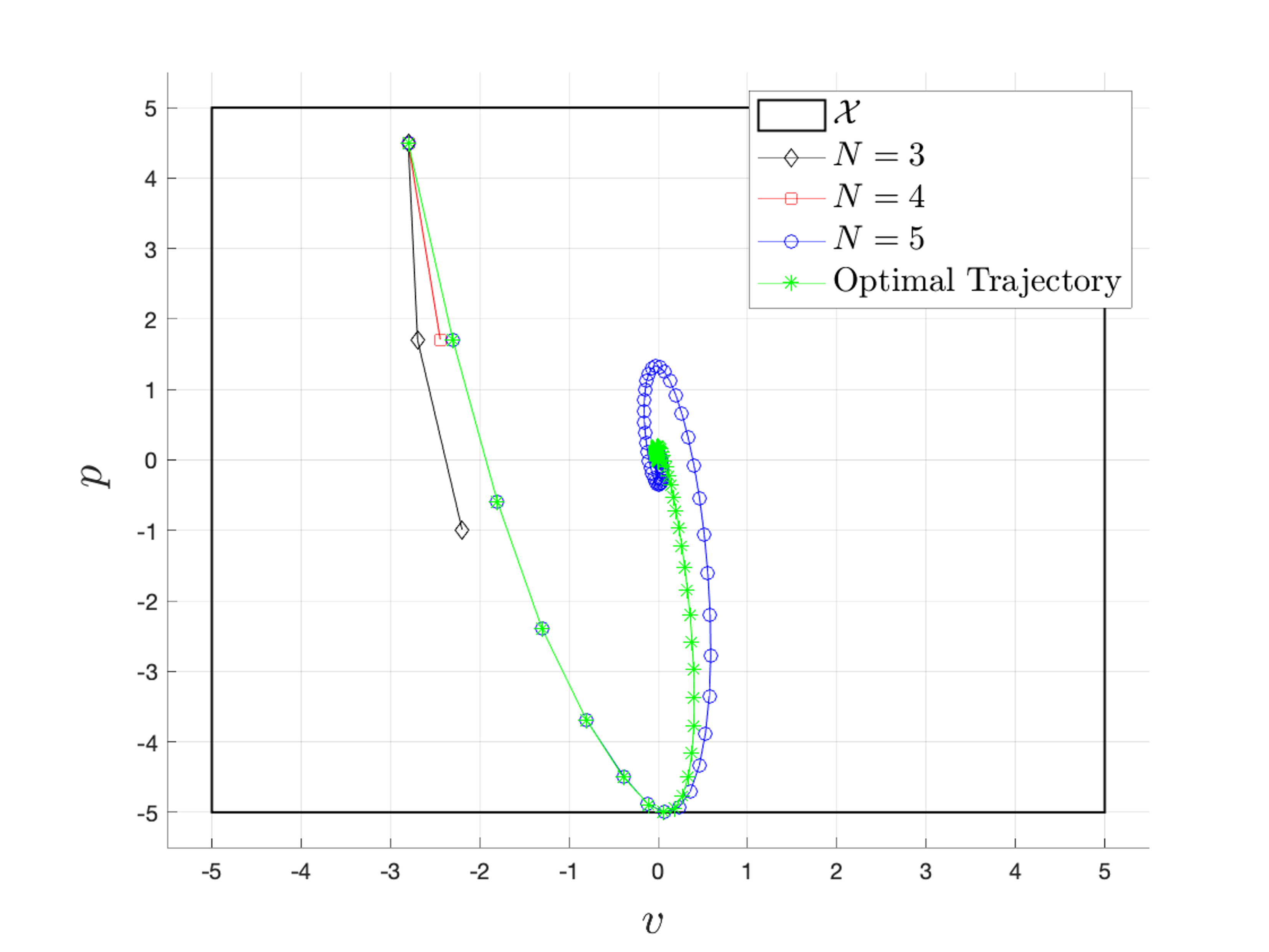
The above figure shows the comparison between the optimal trajectory and the closed-loop trajectories associated with MPC policies designed with \(N \in \{3, 4, 5\}\) and no terminal components. We notice that for \(N=3\) and \(N=4\), the MPC is not able to regulate the system to the origin. In particular, shortsighted control actions steer the drone to a state from which it is impossible remain within the state constraint set \(\mathcal{X}\), i.e., the drone is going too fast towards the floor and collision is inevitable. For this reason, the MPC problem \(J^{MPC}(\cdot)\) becomes unfeasible and the controller fails to regulate the system to the origin. On the other hand, for \(N=5\) the MPC is able to complete the regulation task, but the closed-loop behavior is suboptimal.
Sufficient Conditions for Safety and Stability
To prevent failure caused by shortsighted control actions, we need to appropriately design the terminal constraint set \(\mathcal{X}_N\) and the terminal cost function \(V(\cdot)\). In particular, we should design a terminal constraint set \(\mathcal{X}_N\) which is a \(control\) \(invariant\), i.e.,
\[\forall x \in \mathcal{X}_N \subseteq \mathcal{X}, \exists u \in \mathcal{U} \text{ such that } f(x,u) \in \mathcal{X}_N \subseteq \mathcal{X}.\]The above condition guarantees that the controller does not take shortsighted control actions, which result in safety constraint violations due to inertia and/or limited actuation. In particular, given the optimal predicted input sequence \([u_0^*, u_1^*, \ldots, u_{N-1}^*]\) and associated trajectory \([x_0^*, x_1^*, \ldots, x_N^*]\) with \(x_N^* \in \mathcal{X}_N\), invariance of the terminal constraint set guarantees that there exists a control action \(u \in \mathcal{U}\) such that the following shifted input sequence \([u_1^*, \ldots, u_{N-1}^*, u]\) is feasible for the MPC problem \(J^{MPC}(x(1))\) at the next time step \(t= 1\).
The terminal set ensures that the MPC policy is safe. However, it is not sufficient to guarantee stability of the closed-loop system. Such property may be guaranteed using a terminal cost function which is a \(control\) \(Lyapunov\) \(function\) over the terminal set \(\mathcal{X}_N\), i.e.,
\[\forall x\in \mathcal{X}_N, \exists u \in \mathcal{U} \text{ such that } V(f(x,u)) - V( x ) \leq - h(x,u).\]The above condition guarantees that there exists a feasible control action \(u \in \mathcal{U}\) such that the terminal cost function is decreasing along a trajectory of the closed-loop system. Furthermore, this decreasing property guarantees that the MPC open-loop cost \(J^{MPC}(\cdot)\) is a Lyapunov function for the origin of closed-loop system, i.e.,
\[\begin{align} J^{MPC}(x(t+1)) - J^{MPC}(x(t)) \leq - h( x(t), u(t)), \forall t \geq 0, \end{align}.\]\(J^{MPC}(0)=0\) and \(J^{MPC}(x)\) is radially unbounded. Note that computing a control invariant set and a control Lyapunov function maybe hard also for deterministic linear constrained systems. In practice, these terminal components are computed on a small subset of the state space and they affect the size of the region of attraction associated with the MPC, which is given by the \(N\)-step backward reachable set from the terminal constraint set \(\mathcal{X}_N\).
Optimality Gap
The sufficient conditions that we discussed so far guarantee closed-loop constraint satisfaction and stability. What about optimality? Unfortunately, these conditions are not enough to guarantee optimality of the closed-loop system. In particular, the optimality gap is a function of \((i)\) how well the terminal cost approximates the optimal value function \(J^*(\cdot)\) and \((ii)\) the size of the terminal constraints set, which ideally should be the \(maximal\) \(stabilizable\) \(set\) \(\mathcal{X}_\infty\), i.e., the largest set of states from which the control task can be completed and \((iii)\) the length of the prediction horizon.
To illustrate how the terminal set and terminal cost affect the suboptimality gap we rewrite the optimal value function from the original infinite horizon optimal control problem \(J^*\) described in the Control Problem section as
\[\begin{align} J^*(x(0)) = \min_{u_{0},\ldots, u_{N-1} } \qquad & \sum_{t=0}^{N-1} h(x_{t},u_{t}) + J^*(x_N)\\ \textrm{subject to:} \quad & x_{t+1}=f(x_{t},u_{t}), \forall t\in \{0,\ldots, N-1\}\\ &x_{t} \in \mathcal{X},u_{t}\in \mathcal{U}, \forall t\in \{0,\ldots,N-1\} \\ & x_N \in \mathcal{X}_\infty \\ & x_0=x(0). \end{align}\]Let \([x_0^*, \ldots, x_N^*]\) and \([u_0^*,\ldots, u^*_{N-1}]\) be the optimal solution to the above problem. Now let’s assume that \([x_0^*, \ldots, x_N^*]\) and \([u_0^*,\ldots, u^*_{N-1}]\) is a feasible solution to the MPC problem \(J^{MPC}(x(0))\), then we have that the associated cost is
\[\begin{align} \bar J^{bound}(x(0)) = \sum_{t=0}^{N-1} h(x_{t}^*,u_{t}^*) + V(x_N^*). \end{align}\]Notice that the above cumulative cost is an upper bound on the MPC open-loop cost \(J^{MPC}(x(0))\) and, therefore, we have that
\[\begin{align} J^{MPC}(x(0)) - J^*(x(0)) \leq \bar J^{bound}(x(0)) - J^*(x(0)) = V(x_N^*) - J^*(x_N^*). \end{align}\]Basically, we have that the performance of the MPC policy improves as the terminal constraint \(\mathcal{X}_N\) better approximates the maximal stabilizable set \(\mathcal{X}_\infty\) and the terminal control Lyapunov function \(V(\cdot)\) better approximates the optimal cost function \(J^*(\cdot)\). However computing \(\mathcal{X}_\infty\) and \(J^*(\cdot)\) is as complex as solving the original control problem. In future blog posts, we will discuss how the terminal MPC components can be iteratively synthesized to improve the performance of the MPC.