Model Predictive Control Part II: Learning from data
In the previous blog post, we discussed the importance of the terminal constraint and the terminal cost for MPC design. In this post, we will see that these terminal components can be constructed from historical data.
The Control Problem
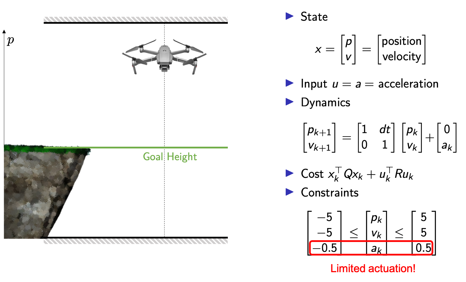
We will consider a regulation problem, where our goal is to control a drone that can move only along the vertical direction. The objective of the controller is to hover in place at a given height. We assume that the drone dynamics are described by a linear system and that the cost is quadratic, as shown in the following figure.
We will use the above example as the system’s state is two-dimensional, and therefore a trajectory of the system can be plotted on a two-dimensional plane. In the following figure, on the two-axis we have the states of the system, i.e., the position and the velocity of the drone.
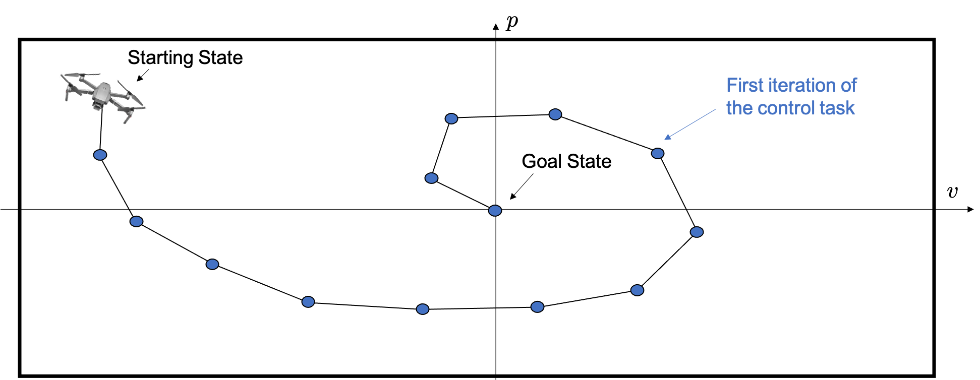
In what follows, we are going to iteratively perform the task of steering the drone from a starting state to the goal state, and we will leverage historical data to improve the performance of the MPC.
Learning Model Predictive Control
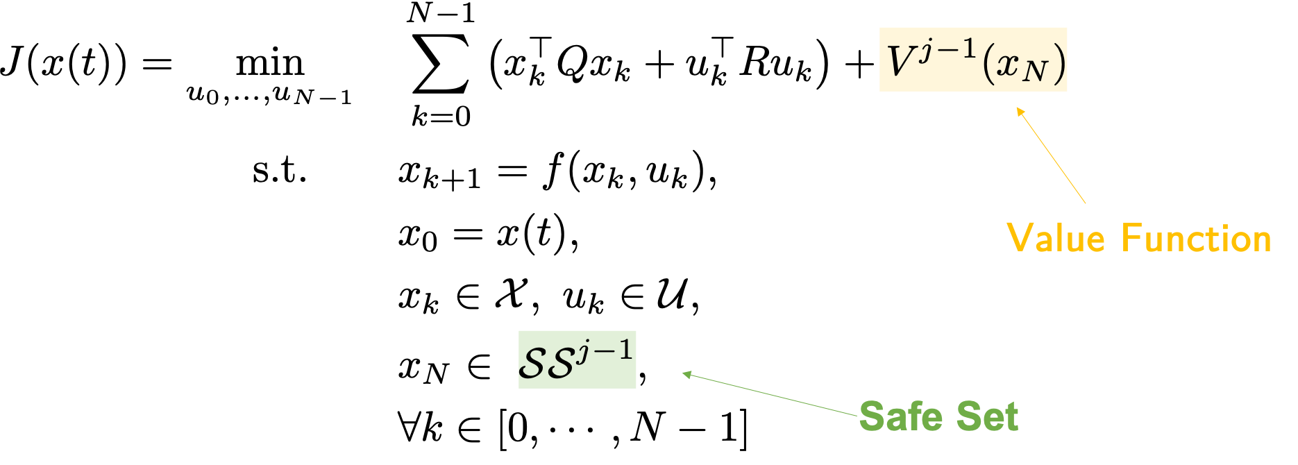
As discussed in the previous blog post, the terminal constraint and terminal cost, often referred to as terminal components, should approximate the tail of the cost and constraint beyond the prediction horizon. The design of these terminal components is crucial to guarantee safety and optimality. In particular, when solving the MPC problem we should use i) a terminal constraint that is given by a safe set of states from which the task can be completed, and ii) a terminal cost function that is a value function representing the cost of completing the task from a safe state.
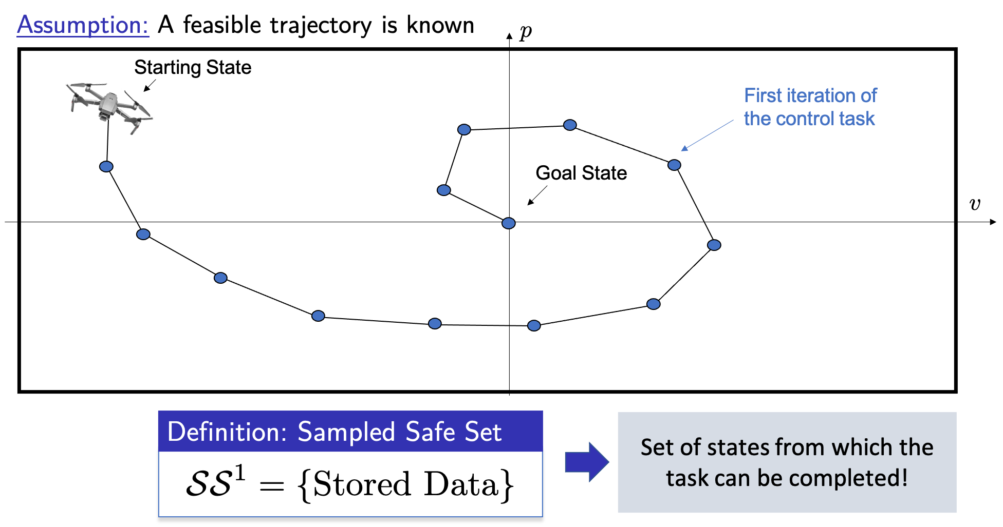
Next, we assume that a first feasible trajectory that is able to complete the task is available and we discuss how to construct safe set and value function approximations.
Building Safe Sets from Data
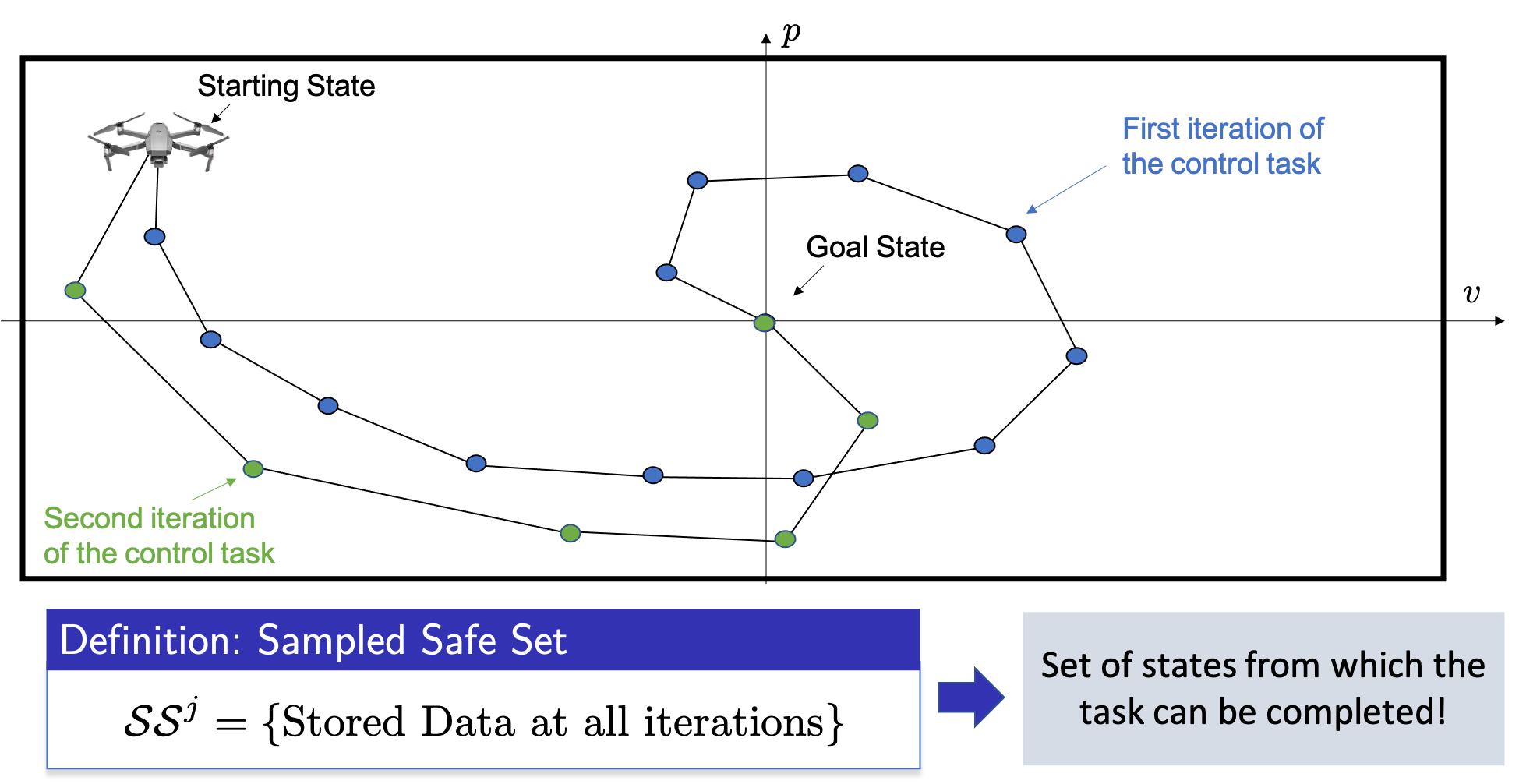
We notice that as the system is deterministic, a state visited during a successful iteration is safe. Indeed, if the system is in a state that we have visited during a successful iteration, we can simply follow the successful trajectory to complete the control task (This fact is trivial for deterministic systems, and for uncertain systems we have to be a bit more careful, please refer to [3]-[4] for further details on uncertain systems). Therefore, we can simply define a safe set of states as the union of the states visited during a successful iteration of the control task.
The safe set \(\mathcal{SS}^1\) can be used as a terminal constraint for our MPC at each time step. In particular, the MPC will plan an open-loop trajectory that steers the system from the current state back to one of the states visited at the previous iteration of the control task. Then, we apply to the system the first control action and the controller plans a new different open-loop trajectory that steers the system back to the safe set. As shown in the following figures, this replanning strategy allows the MPC to steer the drone away from the safe set.
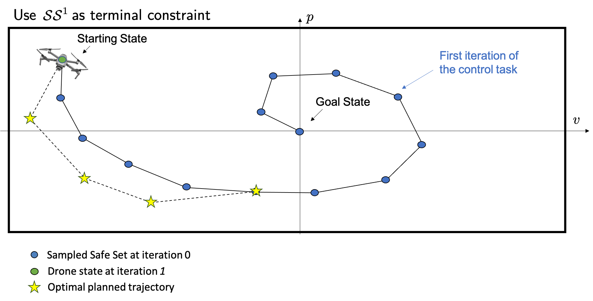
The above figure shows the optimal planned trajectory at time \(t = 0\).
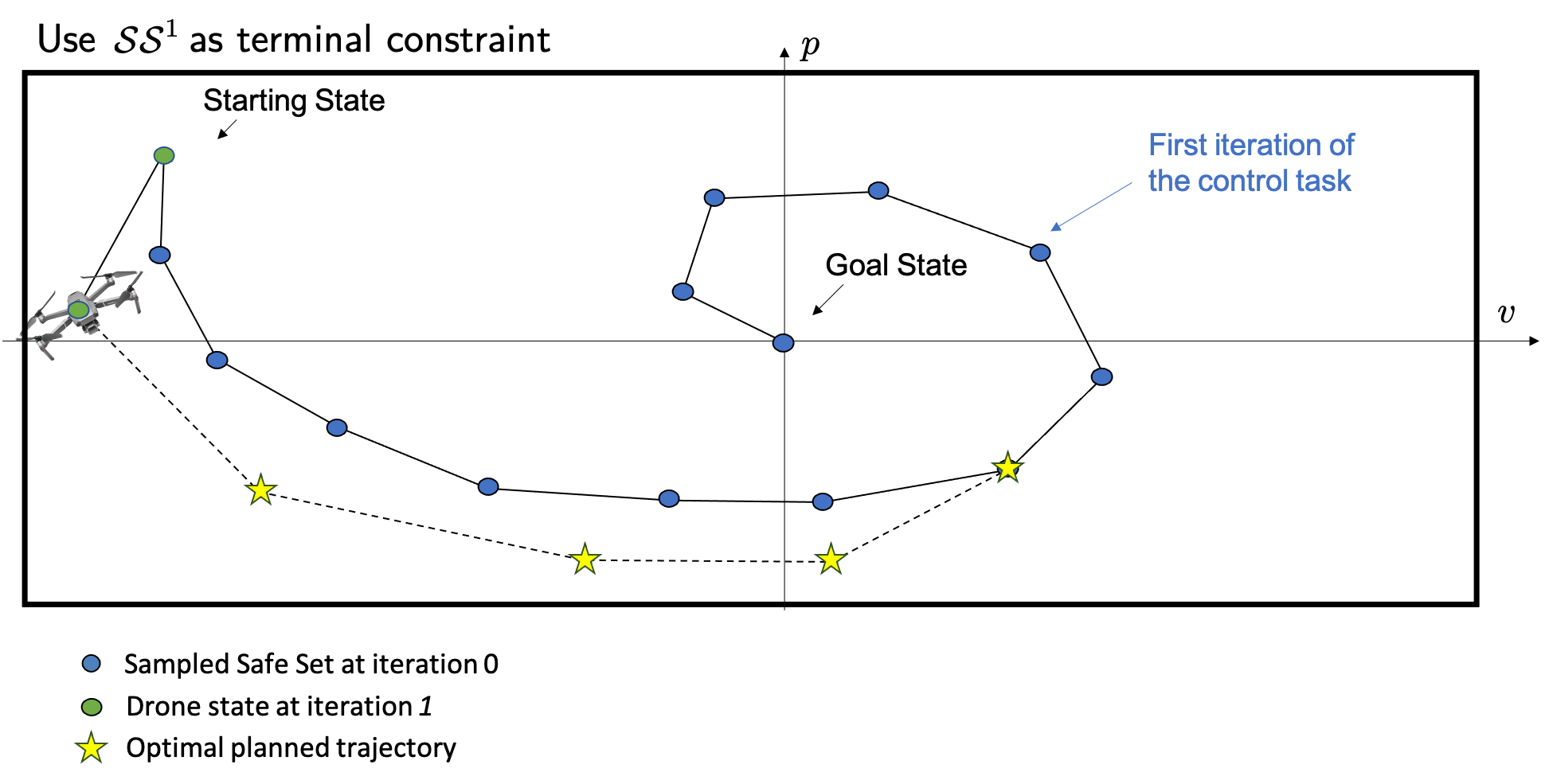
The above figure shows the optimal planned trajectory at time \(t = 1\).
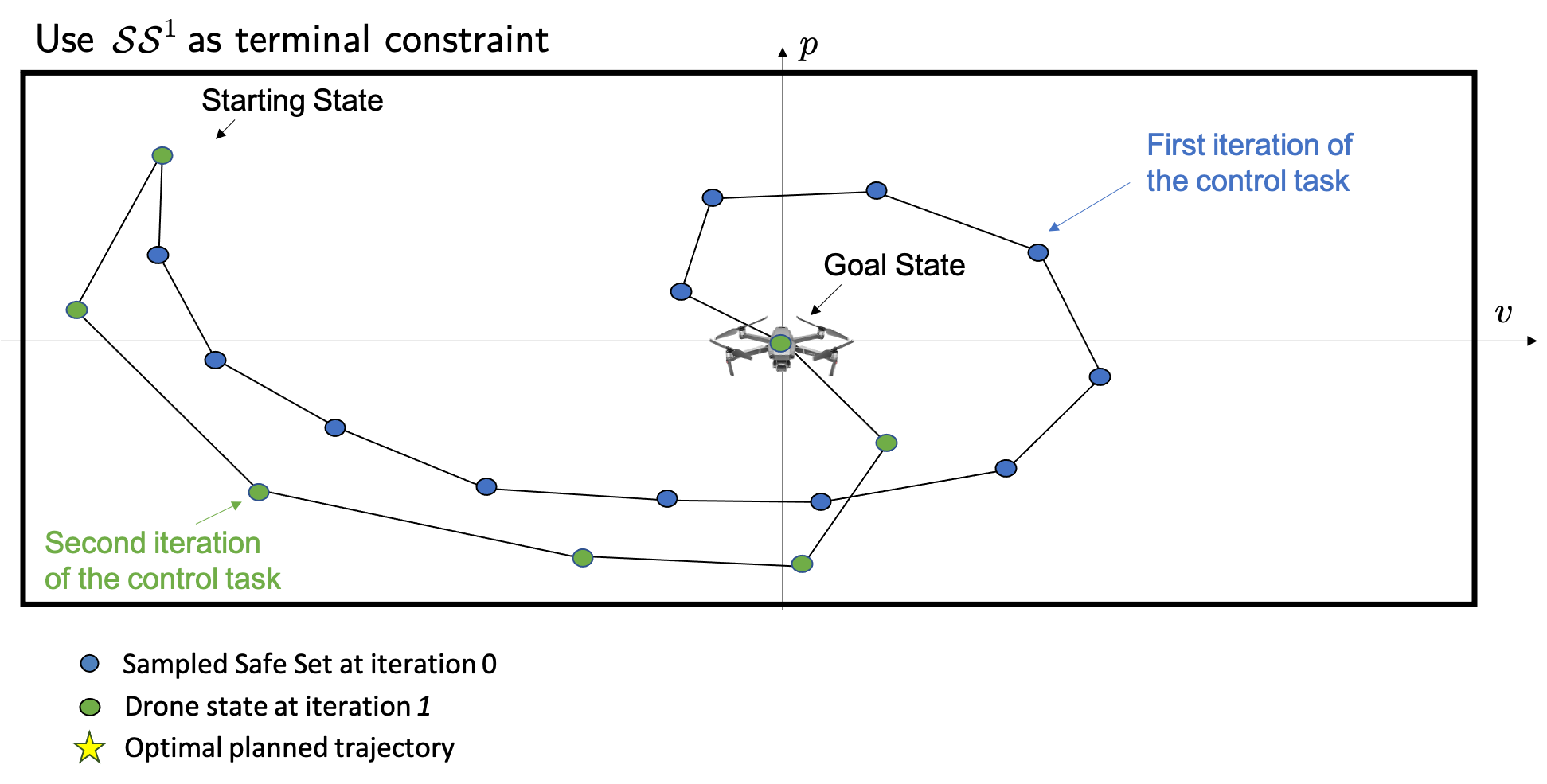
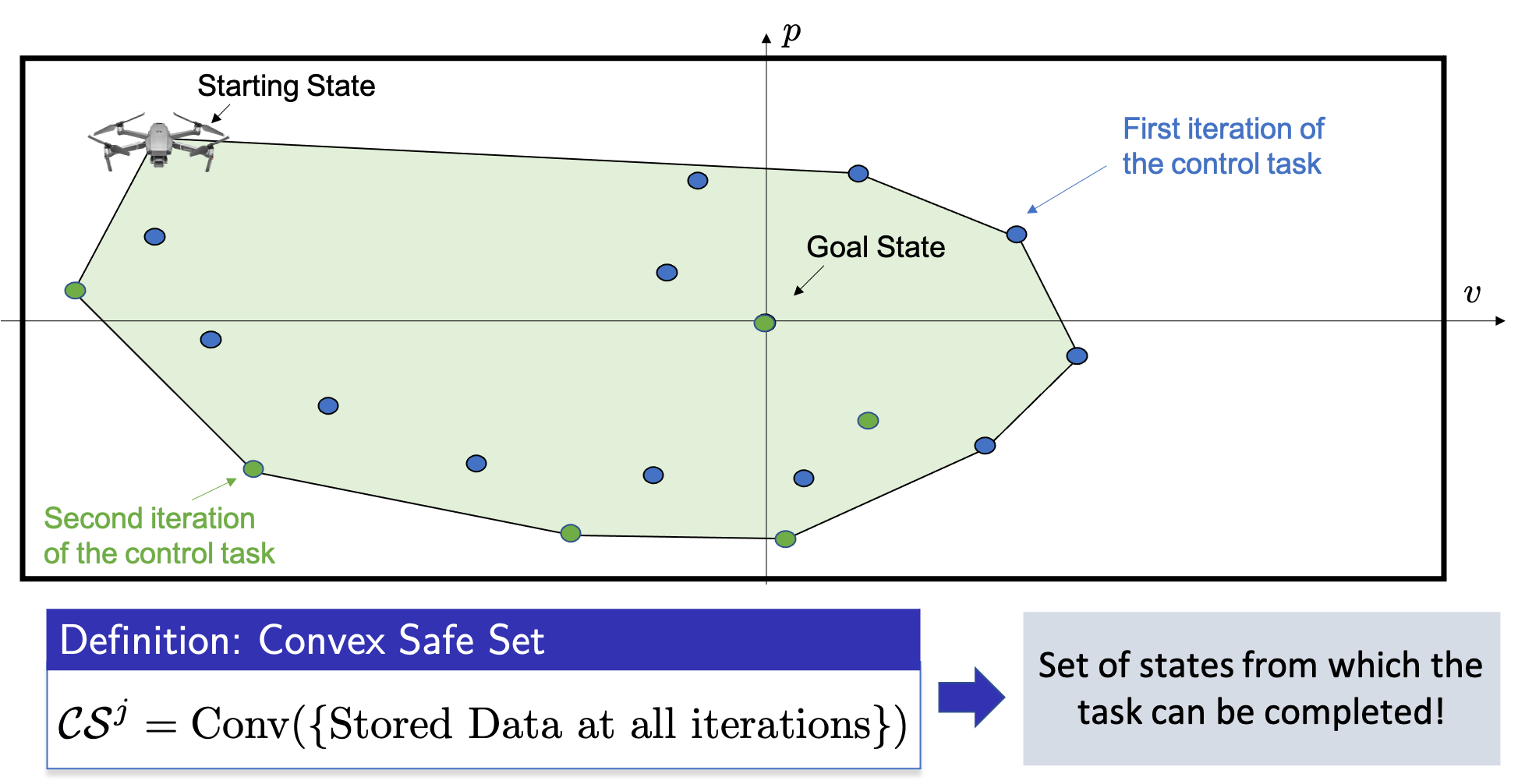
The above figure shows the closed-loop trajectory at the second iteration of the control task. We notice that at the second iteration the controller was able to explore the state space. Therefore, after completion of the second iteration, we can define a bigger safe set which is given by the union of all data points stored during the successful iterations of the control task. In general, we can define the safe set \(\mathcal{SS}^j\) as the union of the states visited across the first successful \(j\) iterations of the control tasks.
However, we notice that the above safe set renders the optimization problem challenging to solve. Indeed, at each time \(t\) the MPC has to plan a trajectory that lands exactly in one of the states that we have visited. Luckily, it turns out that for linear systems also the convex hull of the stored states is a safe set of states from which the task can be completed. Thus, we can define the convex safe set \(\mathcal{CS}^j\) as the convex hull of all stored states up to the \(j\)th iteration of the control task, as shown in the following figure.
Building Value Function Approximations from Data
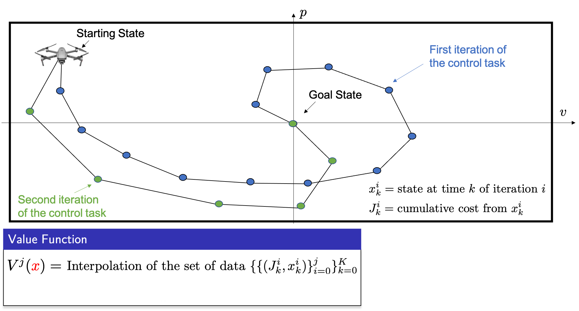
Now let’s see how we can leverage historical data to construct an approximation to the value function. In the following figure, we have two closed-loop trajectories that successfully steered the drone from the starting state to the goal. Let \(x_k^i\) be the state of the system at time \(k\) of iteration \(i\), then we define \(J_k^i\) as the cost of the roll-out from \(x_k^i\). Such roll-out cost can be simply computed by summing up the cost along the closed-loop realized trajectory. Finally, given a data set of costs and states, we define the value function approximation \(V^j\) as the interpolation of the cost over the stored data, as shown in the following figure.
Notice that in the MPC optimization problem the value function will be evaluated at the terminal predicted state, which should belong to the safe region. Therefore, we want to construct a terminal cost function that is defined over the convex safe set \(\mathcal{CS}^j\). For a given state \(x\) in the convex safe set \(\mathcal{CS}^j\), this interpolation can be computed solving a linear program, as shown in the following figure.
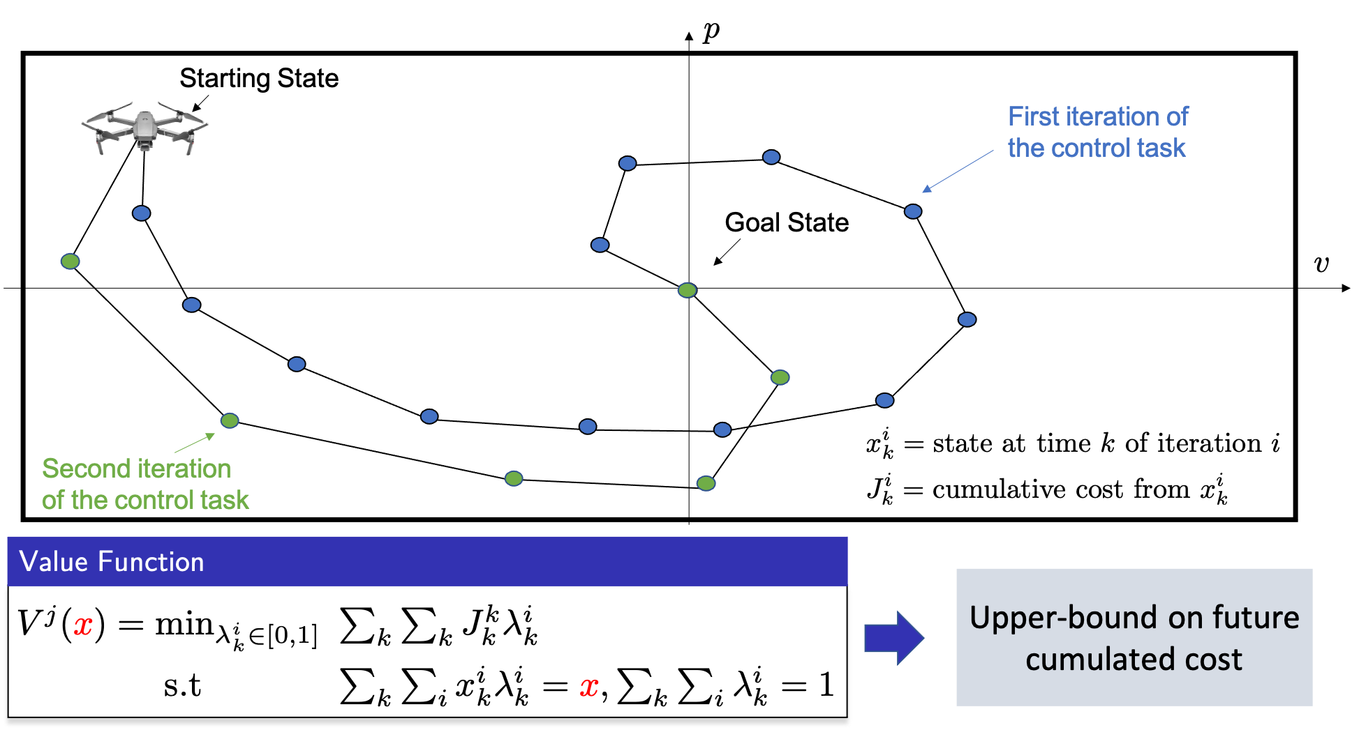
Given the roll-out data, the value function may be approximated also using different strategies. However, there is a main advantage in using a linear program to interpolate the cost associated with the stored states: it can be shown that for linear systems this approximated value function is an upper-bound on the future cumulated cost, for more details please refer to [1].
Computing the Control Action
We have discussed how to leverage historical data to construct the terminal components. Now let’s see how these quantities can be used to compute control actions. Finding an explicit expression for the safe set and value function approximation may be challenging and computationally expensive. However, it turns out that an explicit expression is not needed and we can defined an optimization problem that simultaneously computes the terminal components and the optimal control action. In particular, in the optimization problem we can use a sequence of multipliers \(\lambda_k^i\) that are associated with each data tuple \((x_k^i, J_k^i)\) and are used to represent the safe set \(\mathcal{SS}^{j-1}\) and the value function approximation \(V^{j-1}\), as shown in the following figure.
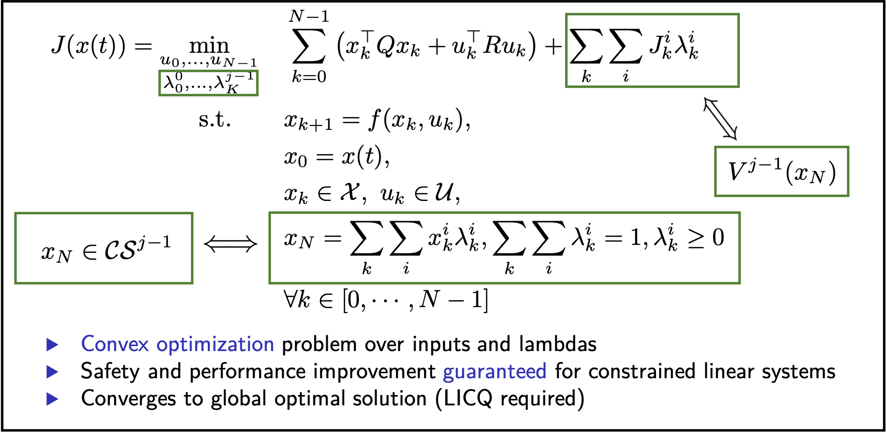
Finally, it is important to underline that for linear systems the above strategy is guaranteed to converge to global optimality when the system dynamics are linear, the constraints polytopic, the cost convex, and a mild technical condition is satisfied [2].
Example and Code
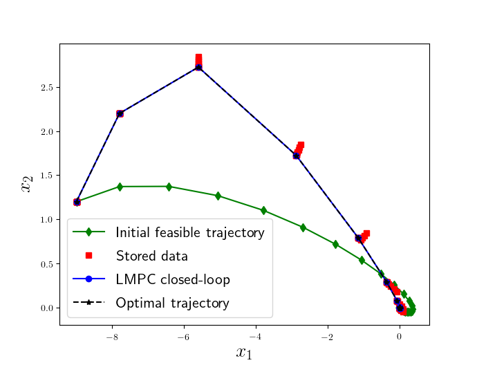
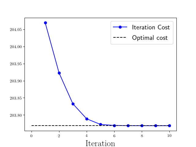
In this GitHub repo, we implemented the learning MPC (LMPC) strategy from [1] and [2] to solve the following constrained LQR problem:

The LMPC improves the closed-loop performance until the closed-loop trajectory converges to a steady-state behavior. In this example, the controller iteratively improves the performance until the closed-loop trajectory converges to the unique global optimal solution to the above infinite time constrained LQR problem. For more details please refer to [1] and [2].
References and code
[1] “Learning Model Predictive Control for Iterative Tasks: A Computationally Efficient Approach for Linear System”, U. Rosolia and F. Borrelli, IFAC World Congress, 2017
[2] “On the Optimality and Convergence Properties of the Learning Model Predictive Controller”, U. Rosolia, Y. Lian, E. T. Maddalena, G. Ferrari-Trecate, and Colin N. Jones. To appear on IEEE Transaction on Automatic Control.
[3] “Robust learning model predictive control for linear systems performing iterative tasks”, U. Rosolia, X. Zhang and F. Borrelli, IEEE Transaction on Automatic Control (2021)
[4] “Sample-Based Learning Model Predictive Control for Linear Uncertain Systems”, U. Rosolia and F. Borrelli, Conference of Decision and Control (CDC), 2019.
LMPC Code available on GitHub